A Duo Traveling Reversely

This blog serves as a memorial for the project titled “Interacting Counter-propagating Flows” to keep notes of why I started and what I’ve learned from it.
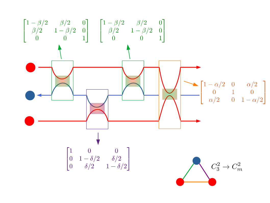
Imagine a scenario that a pair of flows move in opposite directions, and occasionally interact. We want to find out what these interactions lead to, given their initial states. There is no straightforward solution to this problem similar to in a co-propagating scenario. We will clarify the distinct nature of such counter-propagating flows and provide a complete solution to all possible interactions in a system of any size.
What Does Interaction Mean?
In an interaction, two flows are forced to exchange information about their current status (state), leading to immediate changes of status. After this interaction, the flows will move on with the updated status. When this interaction is strong (the strength is tunable from 0 to 1, resembling probability of status transition), the status of flows is expected to be significantly changed toward an average. Remarkably, this interaction is mathematically identical to a well-known stochastic process- Markov process.
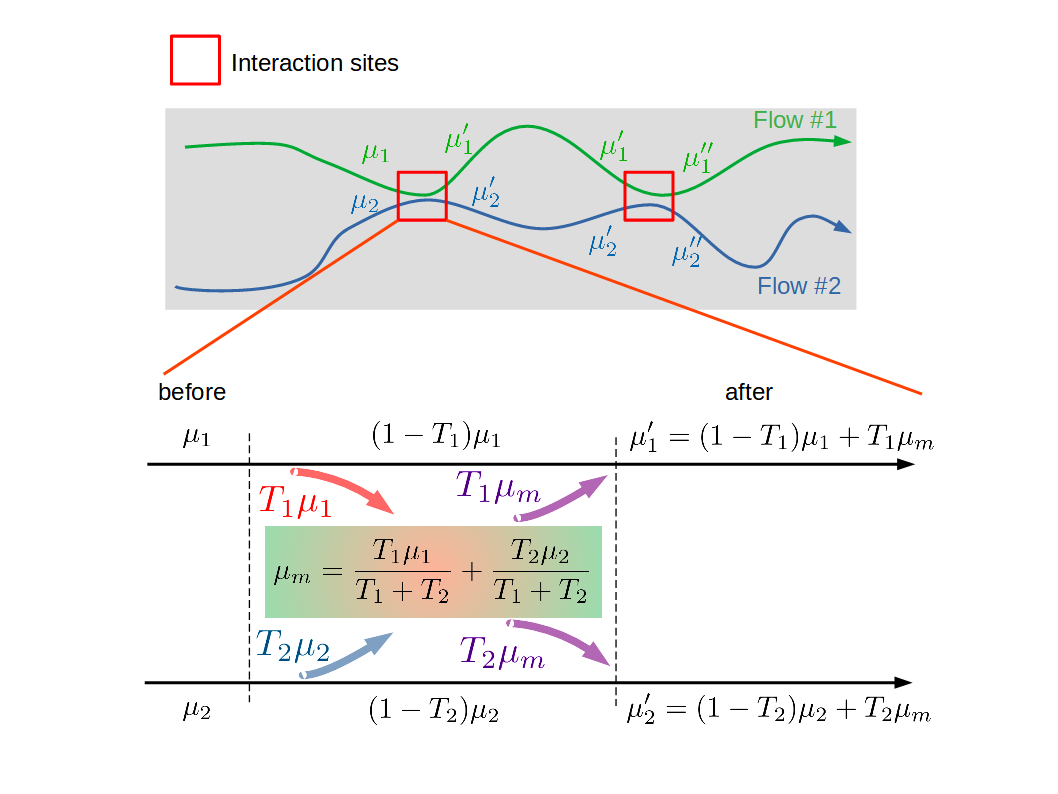
An interaction can be represented by a transmission matrix $M(\beta)$ in which the diagonal elements stand for the probability for remaining in original edge state and off-diagonal elements stand for exchange rate between edge states. This kind of matrix has two important properties: a. All the elements in a row add up to 1; b. All the elements in a column add up to 1. The dimension of this matrix is equal to the number of existing edge states.
\[\mu_1^{\prime}=\left(1-\frac{T_1T_2}{T_1+T_2}\right)\mu_1+\left(\frac{T_1T_2}{T_1+T_2}\right)\mu_2\] \[\mu_2^{\prime}=\left(\frac{T_1T_2}{T_1+T_2}\right)\mu_1+\left(1-\frac{T_1T_2}{T_1+T_2}\right)\mu_2\] \[\begin{bmatrix}\mu_1^{\prime}\\ \mu_2^{\prime}\end{bmatrix} =\begin{bmatrix}1-\beta/2&\beta/2\\ \beta/2&1-\beta/2\end{bmatrix} \begin{bmatrix}\mu_1\\ \mu_2\end{bmatrix}=M(\beta)\begin{bmatrix}\mu_1\\ \mu_2\end{bmatrix}\] \[\beta=\frac{2T_1T_2}{T_1+T_2}\in[0,1]\]Why Are Counter-propagating Flows So Different?
A Sequence of Interactions
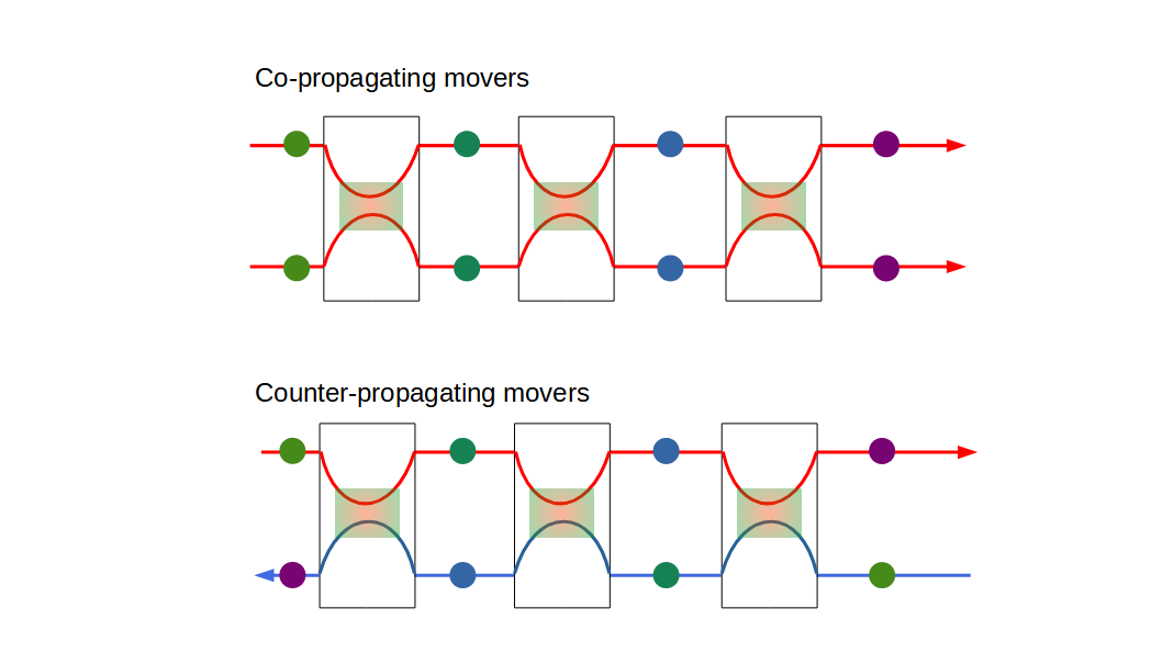
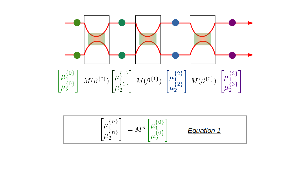
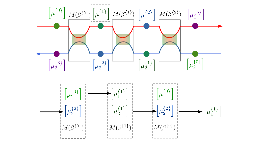
For a single interaction, it is not necessary to distinguish co-propagating and counter-propagating mode. It is only when there are a sequence of interactions along the path, the distinct nature of counter-propagating edge states emerges. For co-propagating edge states, a sequence of interactions is relatively easy to take into account by repeatedly multiplying matrix representation of following interactions from head to end. This is because that the after-status coming out from a former interaction is exactly the before-status for the later interaction. However, this is not true for the counter-propagating situation where keeping track of the current status of each edge state becomes challenging and convoluted.
How to Model a Sequence of Interactions
For co-propagating situation, it is not difficult to see that the combined effect of a sequence of interactions is a product of matrices representing each individual interaction. However, this straightforward approach is not applicable to the counter-propagating situation. We need to be careful in dealing this more complex situation and come up with an algorithm for a minimum system containing two edge states. Unfortunately, this algorithm is not applicable to larger systems (more flows) which involve different types of interactions. Simply speaking, this is due to the fact that the matrix representation of a combined effect should not be structurally similar to any individual interaction matrix. Therefore, we need a general model to deal with arbitrary number of flows and interaction, which will be covered in the next section.
What Happens If More Flows and More Interactions Are Involved
The complexity will increase rapidly when the number of flows and interactions increases. First, introducing more flows means more types of interactions. We simply can not find an analytical format for the combined matrix representation that is structurally identical to any individual matrix representation. In principle, we are still able to provide the analytic form for each matrix element. However, it is almost not writable and solvable by hand once there are more than a few interactions. For doing so, we need a general model that can be transformed into algorithms and implemented in programming language, like Python. To the best of my knowledge, such a general model at this level of complexity is still lacking.
How Can This Be Useful in Physics
Interacting counter-propagating flows are physically realized in a quantum Hall system with edge states moving oppositely. Here I would like to introduce the physics background to illustrate how related research can benefit from this work.
Quantum Hall effect and Its Edge-state Picture
When a two-dimensional (extremely thin film), highly-conducting (high crystalline quality) semiconductor-like material ( e.g., GaAs heterostructure) is subject to a vertically aligned magnetic field (approx. 6 orders of magnitude stronger than Earth’s magnetic field), a profound and intriguing phenomenon, referred to as quantum Hall effect., appears and has been extensively studied since its birth in 1980. In history, several Noble Prizes have been awarded to related discoveries in 1985 , 1998 , 2016. Aside from its deeper physical implication like topology in physics , a well-celebrated, trustful “edge-state” physical picture for this phenomenon is that, electrons are forced to move alongside the thin film edges in one direction, forming dissipationless “edge states” (electron flows). Without delving into deeper theory, a “magic” force seems to guide the motion of electrons. Nevertheless, this simple picture is accurate enough to be applicable in academic discussions and exciting enough to spur expectations of revolution in the field of electric power transmission if no magnetic field is needed (See quantum spin Hall effect).
Landauer-Büttiker Formalism and Interaction between Edge States
Back to “edge states”, this unique “bullet-like” (ballistic) motion of electrons can be most suitably described by a model developed by Markus Büttiker in early 80s based on Rolf Landauer’s earlier work, later referred to as Landauer-Büttiker formalism . Often we do not assume these edge states interact with each other or exchange electrons. In a typical device with terminals (electron reservoirs), interactions between edge states are in principle not discernible if all edge states move in the same direction (a co-propagating mode). This is because that co-propagating edge states themselves are identical in terms of physical properties like electrochemical potential and any exchange between them would not lead to any observable consequence. In order to detect this type of interaction, dedicated device design is needed to divert co-propagating edge states into different paths. For counter-propagating edge states, this interaction is directly measurable even in a standard device (uniform path).
Code Implementation
The source code of this open-source project is currently host on Github
Design of Classes
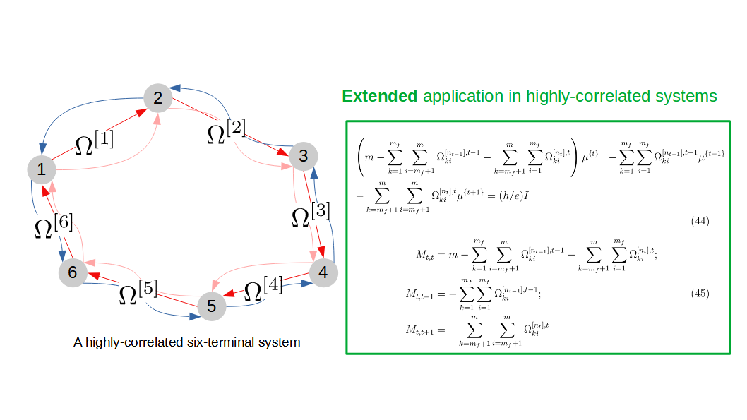
For python implementation, two classes are designed: System and Edge. In class Edge, a method trans_mat is built to implement the forward-propagation process and to return a matrix representation of combined effect of the interaction sequence represented by this Edge instance. Another method status_check is built to implement the forward- and back- propagation processes together to return all the status along the sequence. To initialize an instance of class system, we need to first initialize several Edge instances as input beforehand. This system class account for a real system that contains not only sequences of interactions but also terminals which separate edges. A method mastermat is designed to return the master matrix equation and another method solve will return its solution - a vector of terminal voltages.
Dynamic Programming for Diverting Edge States
I would like to highlight the implementation of dynamic programming, which allows for diverting edge states into different paths. In a standard Landauer-Büttiker system, all edge states enter each terminal without exception. The electronic measurement is only performed via terminals which measure all edge states at once. Consequently, this measurement result is an average of all edge states in terms of electro-chemical potential.
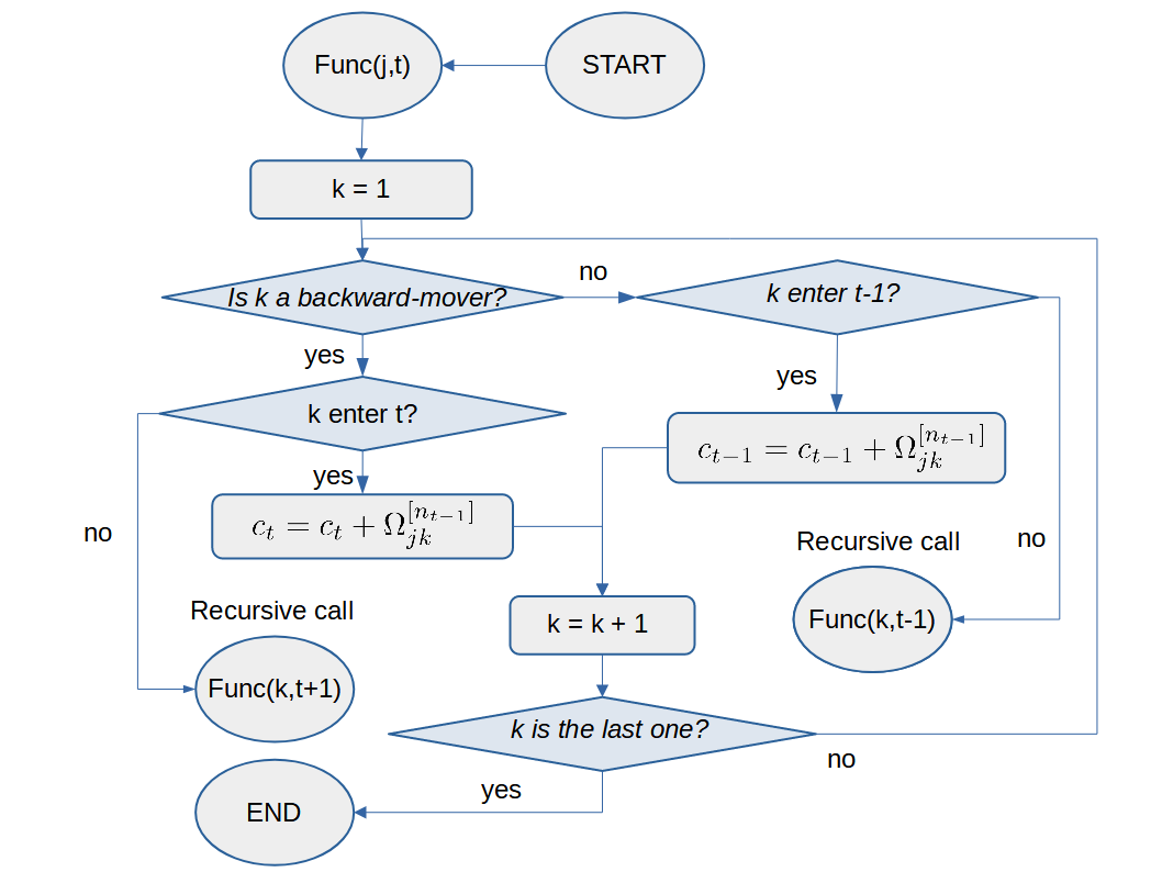
To extract additional information of edge states, it is advisable to block some of them from entering particular terminals, leading to different paths. In other words, this additional controls imposed on edge states may reveal hidden information, not detectable in conventional configuration (standard Landauer-Büttiker system). However, a complex blockage pattern may also cause difficulty in defining the blocked edge state, because that the information carried by these edge states, not detectable by terminals, spread into other edge states via interactions directly or indirectly. An algorithm is developed to resolve this complexity recursively.
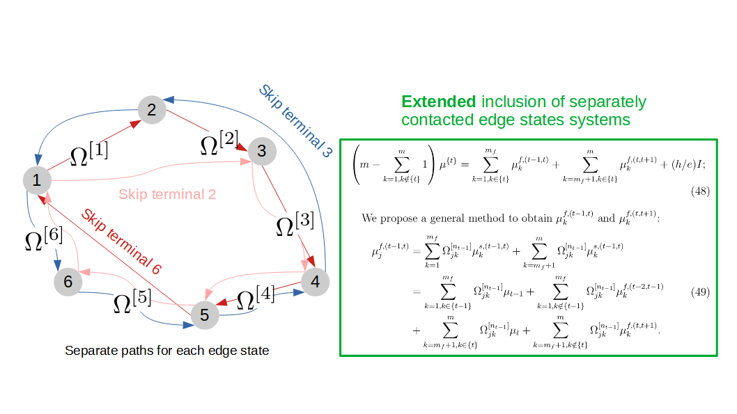
An algorithm is developed to resolve this complexity recursively.
Usage
The design principle for usage is to facilitate the bottom-up construction of a system from the building block - interaction. Hereby I would like to introduce how to build a system step-by-step with existing infrastructure from package counterfusion.
A single interaction can be defined with a python snippet below:
from counterfusion import interaction_builder
left_stochastic_matrix = interaction_builder(dim=2,id1=0,id2=1,value=[0.1,0.3])
right_stochastic_matrix = left_stochastsic_matrix.T
doubly_stochastic_matrix = interaction_builder(dim=2,id1=0,id2=1,value=0.5)
An edge containing a sequence of interactions can be defined:
from counterfusion import generate_bynumber, Edge
#===============================================================
# General information for the edge - Hyperparameters
totalNumMover = 4
numForwardMover = 2
initStates = [1,1,0.2,0.2]
#===============================================================
# Information of scattering events
# Interaction parameters
v03 = 0.3
v01 = 0.5
v23 = 0.8
edgeDef = [[0,3,v03,10],[0,1,v01,10],[2,3,v23,10]]
edgeInfo = generate_bynumber(edgeDef)
edge = Edge(edgeInfo,totalNumMover,numForwardMover)
A six-edge (terminal) system can be defined:
from counterfusion import *
# Define a six-terminal system
# C1--M1--C2--M2--C3--M3--C4--M4--C5--M5--C6--M6--C1
# Total number of edge states: 4
# Number of forward-moving edge states: 2 (#0,#1)
# Number of backward-moving edge states: 2 (#2,#3)
#===============================================================
# General information for the system - Hyperparameters
totalNumMover = 4
numForwardMover = 2
zeroVoltTerminal = 3
#===============================================================
# Information of scattering events
# Interaction parameters
v02 = 0.9
v13 = 0.7
v12 = 0.3
# Define interaction between nodes (contacts)
# C1--M1--C2
edgeDef1 = [[0,2,v02,10],[1,3,v13,10]]
# C2--M2--C3
edgeDef2 = [[0,2,v02,10],[1,2,v12,10]]
# C3--M3--C4
edgeDef3 = [[0,2,v02,10],[1,3,v13,10]]
# C4--M4--C5
edgeDef4 = [[0,2,v02,10],[1,2,v12,10]]
# C5--M5--C6
edgeDef5 = [[0,2,v02,10],[1,3,v13,10]]
# C6--M6--C1
edgeDef6 = [[0,2,v02,10],[1,2,v12,10]]
#================================================================
edgesDef = [edgeDef1,edgeDef2,edgeDef3,edgeDef4,edgeDef5,edgeDef6]
edgesInfo = []
for edgeDef in edgesDef:
    edgesInfo.append(generate_bynumber(edgeDef))
graph = []
for edgeInfo in edgesInfo:
    graph.append(Edge(edgeInfo,totalNumMover,numForwardMover))
nodesCurrent = [1,0,0,-1,0,0]
sys = System(nodesCurrent,graph,numForwardMover,zeroVoltTerminal)
Separate paths of edge states can be realized by editing blockStates:
# The definition of blocking_state should strictly follow this rule:
# [[index_of_terminal#1,[all blocked states in this terminal]],[[index_of_terminal#2,[all blocked states in this terminal],...]]]
blockStates = [[1,[0]],[0,[2]],[2,[3]],[3,[1]]]
sys = System(nodesCurrent,graph,numForwardMover,zeroVoltTerminal,blockStates)